Introduction.
Temporal analysis often requires measuring dependence between two heterogeneous data types: a continuous time series, such as sales or traffic volume, and a temporal event sequence, such as holidays, promotions, or system states. Existing measures do not directly fit this setting: Pearson correlation assumes two continuous signals, while pointwise mutual information is typically defined for discrete events.
We introduce HUMI (Mutual Information between Time Series and Temporal Event Sequence), a method for directly estimating mutual information between a time series and a temporal event sequence. HUMI produces a single dependence score analogous to Pearson correlation and supports downstream tasks including lag and causality analysis, seasonality measurement, repeated-pattern discovery, covariate selection, and feature selection.
Existing approaches, however, do not reach this combination of accuracy and generality: they usually run into one of two gaps:
Neural estimators need many matched time series and event sequence pairs, but these pairs are expensive to label by hand and rarely exist as ready to use data.
Existing non-cross-modal measurement approaches often rely on ad hoc data transformations, and existing MI estimators struggle with rounded values, repeated measurements and redundant event states.
Neither gap is addressed directly, so existing methods cannot produce a reliable estimate, which raises a basic question: can we trust the estimated interaction score?
This kind of interaction estimate shows up across many research problems and settings, so an unreliable score causes trouble throughout downstream analysis. A few examples:
Time-delayed mutual information (TDMI) can measure lagged dependence, but existing methods are not built to directly measure cross-modal causality strength between a time series and an event sequence.
Classical methods can detect seasonality, but noisy or disrupted data can distort the result. Even when they find seasonality, they may not tell how much noise or deviation from a clean seasonal pattern is present.
Seasonality is a global repeated pattern at a fixed interval across the whole series. A local pattern that holds only under certain conditions, such as a specific month, could be measured by manually splitting the series first, but no existing tool measures it directly.
Forecasting often needs discrete covariates such as promotions, holidays or calendar attributes, ranked by how strongly each one relates to a continuous target like sales. Existing methods can already do this, but only after cutting the continuous target into bins first, and that binning step can distort the ranking.
These tasks may look different, but they share the same missing piece. HUMI addresses it by combining three key ideas:
It provides a theoretical estimation foundation for mutual information between discrete and continuous variables, without forcing one side to become the other.
It models a recorded time series as both continuous variation and repeated value mass caused by finite measurement precision.
It groups similar event states together, so repeated or overlapping event information does not overweight the final score.
Together, these components provide a more reliable measure of heterogeneous temporal dependence.
Background and related work.
Most existing dependence measures assume homogeneous inputs. A common workaround is to transform one data type into another, for example by discretizing continuous values,2 assigning numerical codes to event labels,3 or decomposing event states into binary variables. Such transformations can distort the result: binning may create or hide dependence, numerical codes may impose artificial ordering, and binary decomposition may lose the structure of the original event sequence.
Mixed discrete-continuous mutual-information estimators5,3 avoid some of these transformations, but they remain sensitive to repeated values caused by finite measurement precision and to redundant or highly correlated event states. Neural estimators offer greater flexibility,6 but require large collections of aligned time-series and event-sequence pairs and may produce dataset-dependent, difficult-to-interpret scores.
These limitations directly affect downstream tasks. Lag analysis requires reliable dependence estimates across temporal shifts,8 seasonality and repeated-pattern analysis require distinguishing strong patterns from noisy or conditional ones,9, 10, 11 and covariate selection requires consistently ranking discrete temporal factors.12,13 HUMI estimates dependence directly from a single observed pair, without binning or learned cross-modal representations, while explicitly accounting for repeated measurements and event redundancy.
1. Church and Hanks, Word Association Norms, Mutual Information, and Lexicography, 1990.
2. Liu et al., Discretization: An Enabling Technique, 2002.
3. Ross, Mutual Information between Discrete and Continuous Data Sets, 2014.
4. Luo et al., Correlating Events with Time Series for Incident Diagnosis, KDD 2014.
5. Kraskov et al., Estimating Mutual Information, 2004.
6. Belghazi et al., Mutual Information Neural Estimation, 2018.
7. Radford et al., Learning Transferable Visual Models From Natural Language Supervision, 2021.
8. Fraser and Swinney, Independent Coordinates for Strange Attractors from Mutual Information, 1986.
9. Box et al., Time Series Analysis: Forecasting and Control, 2015.
10. Cleveland et al., STL: A Seasonal-Trend Decomposition, 1990.
11. Brillinger, Time Series: Data Analysis and Theory, 2001.
12. Guyon and Elisseeff, An Introduction to Variable and Feature Selection, 2003.
13. Belmonte et al., Hierarchical Shrinkage in Time-Varying Parameter Models, 2014.
14. Dougherty et al., Supervised and Unsupervised Discretization of Continuous Features, 1995.
Approach.
HUMI starts by turning the temporal question into a dependence question. For each aligned pair, X is the event state, such as weekday, holiday, promotion or medication status, and Y is the corresponding signal value, such as traffic volume, sales, temperature or heart rate. In simple terms, we ask: how much does knowing the event state reduce uncertainty about the signal value?
The core object is the paper's mutual information formulation for one discrete variable and one continuous variable. The estimator computes this quantity through entropy terms: the event probabilities come from empirical frequencies, while the signal distribution is estimated nonparametrically. Instead of predicting the next signal value, HUMI measures dependence directly, which keeps it closer to a measurement operator than to a trained classifier, embedding model or forecasting model.
I(X, Y) = Σx∈X ∫y∈Y p(x,y) log( p(x,y) / (p(x)p(y)) ) dy
MI is high when knowing X makes Y less uncertain.
Two modeling details make this practical for real temporal data. First, a recorded time series is not always a clean continuous curve. Take temperature as an example: the real temperature changes continuously, but a sensor may only report one decimal place, so many timestamps can share the exact same value, such as 20.1, 20.1 and 20.2. Classical nearest-neighbor entropy estimators are designed for continuous samples, where exact duplicates should almost never happen. When duplicates appear, the nearest-neighbor distance can become zero, and the estimate becomes unstable. HUMI handles this with continuous-discrete duality: values that appear once are estimated as continuous samples, while repeated values are treated as repeated recorded states. This keeps the numeric meaning of the signal without pretending that duplicated readings are ordinary continuous samples.
Second, event sequences often contain labels that are different symbols but lead to similar signal behavior. For example, two promotion types in a sales dataset, or two calendar states in a traffic dataset, may produce similar distributions of aligned signal values. Treating every raw event label as fully separate can fragment the data and make the estimate unstable. HUMI optionally collects the aligned signal values for each event type, compares those empirical conditional distributions, and uses hierarchical clustering to replace redundant labels with latent event groups before estimating MI.
As a result, the estimator keeps the two modalities close to their native forms: the signal remains numeric, the event sequence remains categorical, and the final output is a normalized MI score for ranking event sequences, discovering lags and selecting covariates.
What makes the estimator robust:
Unique values use continuous entropy; repeated values become discrete mass.
Event labels with similar signal distributions can share one latent label.
Pseudocode
Downstream tasks.
The experiments ask whether one score can work as a practical dependence operator whenever a continuous signal must be compared with discrete temporal context.
We start from seasonality because it is the classic version of this problem. Traditional methods are good at finding a period, but they usually treat seasonality as a global signal pattern and can be hard to interpret when noise, missing values or holidays weaken the cycle. HUMI improves this by turning seasonality into a dependence score between the time series and calendar context: it can still identify the period, but it also says how strong the seasonal effect is. From there, the same idea leads to a more general temporal repeated pattern task, where repetition can depend on local context rather than a single global cycle.
The remaining tasks test the same idea in other settings: cross-modal TDMI measures delayed dependence between events and signals, covariate selection ranks discrete forecasting covariates for a continuous target, and feature selection shows that the estimator can also work outside temporal data when the input is simply continuous values paired with discrete labels.
Seasonality with strength
Classical tools such as ACF, seasonal decomposition and Fourier analysis are good at searching for a fixed period. But they mostly answer a yes or no style question: is there a dominant period? Real traffic is messier. Holidays, missing values and irregular disruptions can blur the pattern, while decomposition can still report a strong weekly cycle even when the observed signal is clearly partly broken.
HUMI treats seasonality as dependence between traffic volume and calendar context. This keeps the familiar weekly seasonality task, but adds a more useful score: it detects the 7 day pattern and also reflects how strongly that pattern appears. In the paper, June-July receives a higher MI score than December-January, matching the visual fact that winter traffic is more disrupted by holidays.
Dataset
Minneapolis daily traffic volume. The event sequence is day-of-week labels. June-July has clearer weekly seasonality; December-January is disrupted by holidays.
Baselines
ACF, seasonal decomposition plus ACF and Fourier transform. These methods mainly detect a candidate period.
Result
HUMI finds the same 7-day pattern in both periods, but the score drops from 0.6501 to 0.5664 when the pattern becomes weaker.
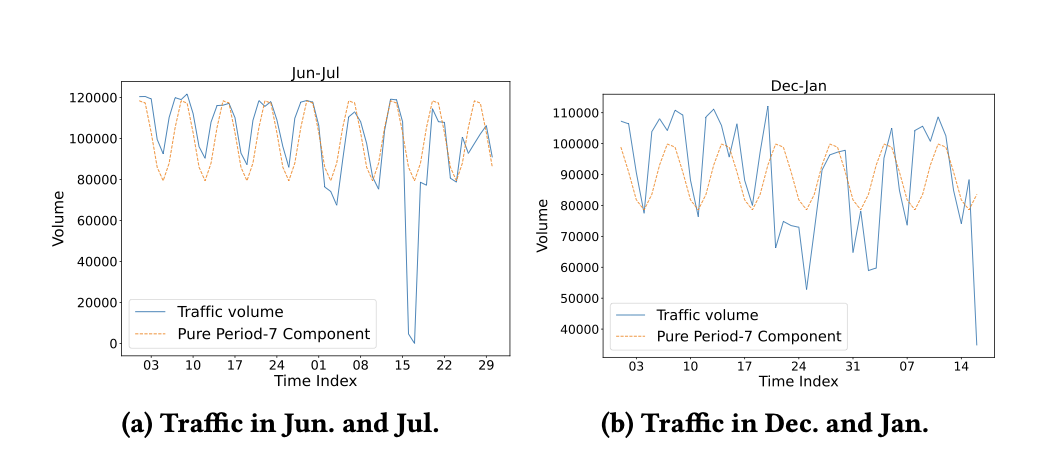
| Data | Method | Measure | Seasonality |
|---|---|---|---|
| Jun-Jul | ACF | 0.4651 | No |
| Jun-Jul | SD+ACF | 0.9817 | 7 days |
| Jun-Jul | FT | 0.13 | 7-8 days |
| Jun-Jul | Ours | 0.6501 | 7 days |
| Dec-Jan | ACF | 0.2181 | No |
| Dec-Jan | SD+ACF | 0.9157 | 7 days |
| Dec-Jan | FT | 0.08 | 11-12 days |
| Dec-Jan | Ours | 0.5664 | 7 days |
ACF and FT can miss or drift under noise. SD+ACF detects weekly seasonality but stays close to 1 even when holidays disrupt the pattern; HUMI gives a lower score for the disrupted period.
General repeated patterns
After seasonality, HUMI extends repeated pattern analysis beyond one global fixed period. A local repeated pattern may appear only under specific contextual conditions, rather than across the whole series as a single periodic structure. This is why HUMI uses temperature as the next experiment: day/night labels provide a coarse temporal context, while combining month with day/night gives a finer context. The finer context narrows the possible temperature range, so the repeated pattern becomes stronger and easier to quantify.
This is where normalized MI is useful. If the event context explains the signal better, the score should increase in a stable and interpretable way. In the temperature experiment, richer contexts move from DN to TwoMon to DNTwoMon, and HUMI increases monotonically from 0.6124 to 0.8932 to 0.9596.
Dataset
Minneapolis 2023 air temperature sampled at 12-hour intervals. Event sequences describe day/night, two-month blocks and their joint context.
Baselines
Ross gives negative values, violating MI non-negativity. Mixture stays positive, but its scale is unbounded, making it hard to tell whether different contextual constructions are strong enough.
Result
As the context becomes richer, HUMI increases from 0.6124 to 0.8932 to 0.9596, giving a bounded score for local repeated patterns.
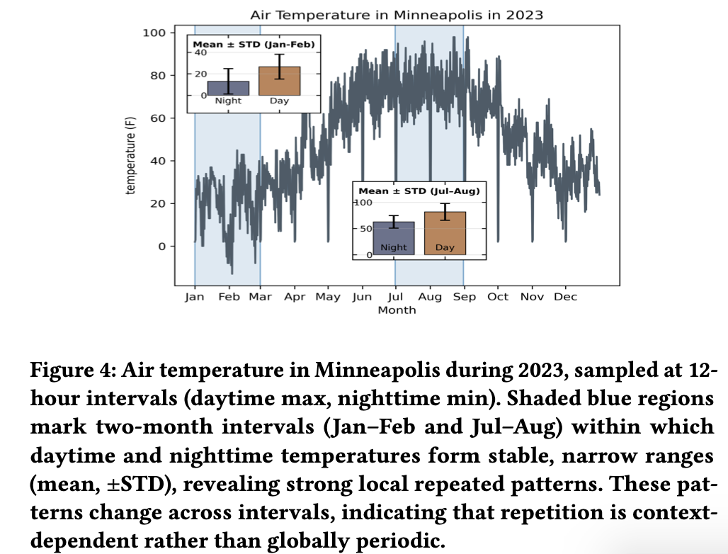
| Method | DN | TwoMon | DNTwoMon |
|---|---|---|---|
| Ross | -1.8418 | -0.7864 | -0.2332 |
| Mixture | 0.3749 | 1.2807 | 1.5544 |
| Ours | 0.6124 | 0.8932 | 0.9596 |
The score increases as the temporal context becomes more informative, while Ross gives invalid negative values and Mixture is unbounded.
Cross-modal TDMI
TDMI measures delayed dependence, which is useful for causality analysis. The usual setting compares two continuous time series. HUMI changes the input pair: it can compare an event type at time t with a continuous signal value at time t + tau, without turning either side into the other.
Dataset
Synthetic event sequence with three event types. Each event controls a different Gaussian distribution for the signal at a true delay of tau = 5.
Baselines
Series2Seq and Seq2Series force the data into one type; Ross and Mixture estimate discrete-continuous MI but do not fully handle repeated rounded values.
Result
HUMI recovers the delay peak at tau = 5 and closely matches the ground truth, showing that continuous-discrete duality improves stable TDMI estimation.
| Lag | Ground Truth | Ours |
|---|---|---|
| 0 | 0.0376 | 0.0353 |
| 5 | 1.0984 | 1.0988 |
| 9 | 0.0384 | 0.0355 |
The estimator recovers the true delayed dependence peak without converting event labels into numbers or discretizing the signal.
Covariate selection
Forecasting often needs discrete covariates such as promotions, holidays or calendar attributes. The missing tool is a direct way to rank those event covariates for a continuous target series before training a forecasting model.
Dataset
Rossmann and M5 sales forecasting. The target is a continuous sales time series; candidate covariates are discrete event or calendar attributes.
Baselines
Ross and Mixture are used to rank covariates by MI. Forecasting models then test whether the selected covariates actually help downstream prediction.
Result
Ours-Cluster gives the best NDCG in nearly all settings, showing that grouping redundant discrete states improves covariate ranking.
| Model | Dataset | Ours | Ours-Cluster |
|---|---|---|---|
| CatBoost | Rossmann | 0.94 | 0.95 |
| CatBoost | M5 | 0.81 | 0.86 |
| DeepAR | Rossmann | 0.90 | 0.92 |
| DeepAR | M5 | 0.76 | 0.82 |
| Chronos-2 | Rossmann | 0.92 | 0.95 |
| Chronos-2 | M5 | 0.78 | 0.83 |
Feature selection
HUMI was motivated by temporal data, but the estimator itself does not depend on the order of instances. It only needs paired samples from a continuous variable and a discrete variable. This means the same formulation can be used for tabular feature selection: a continuous feature becomes the continuous variable, and the class label becomes the discrete variable.
Dataset
Mixed-type tabular classification datasets. Each continuous feature is paired with a discrete class label and ranked by mixed MI.
Baselines
Ross and Mixture are compared as MI-based feature selectors. Selected features are evaluated through RF, SVM and logistic regression.
Result
HUMI wins against Ross and Mixture in most settings, and clustering usually improves the ranking by reducing redundant feature-label information.
| Comparison | Win | Tie | Lose | Interpretation |
|---|---|---|---|---|
| Ours vs Ross | 89 | 14 | 17 | Ours wins more often. |
| Ours vs Mixture | 93 | 15 | 12 | Strongest pairwise result. |
| With cluster vs Without cluster | 77 | 20 | 23 | Clustering usually helps. |